Here's more stuff on the 600 uniformly distributed numbers exercise. For the "discrete" case (i.e. whole numbers / integers), you use 0.5 to 6.5 and the round function.

Variable    N  N*    Mean  SE Mean   StDev  Minimum      Q1  Median      Q3  Maximum
C2        600   0  3.5033   0.0699  1.7112   1.0000  2.0000  3.0000  5.0000  6.0000

For the "continuous" case, you use 0.5 to 6.5 and use the column of numbers directly (don't round).

Variable    N  N*    Mean  SE Mean   StDev  Minimum      Q1  Median      Q3  Maximum
C1        600   0  3.4974   0.0707  1.7325   0.5073  2.0086  3.4566  4.9780  6.4891

The theoretical standard deviation for a *discrete* uniform distribution is sqrt(((6-1+1)*(6-1+1)-1)/12)=sqrt((6*6-1)/12)=sqrt(35/12)=1.70782512766. It can be seen that the standard deviation from Minitab (1.7112) and the theoretical standard deviation (1.70782512766) are very close.

The theoretical standard deviation for a *continuous* uniform distribution is (6.5-0.5)/sqrt(12)=1.73205080757. It can be seen that the standard deviation from Minitab (1.7325) and the theoretical standard deviation (1.73205080757) are very close.

Note! The formulas are slightly different for the *discrete* and *continuous* cases.

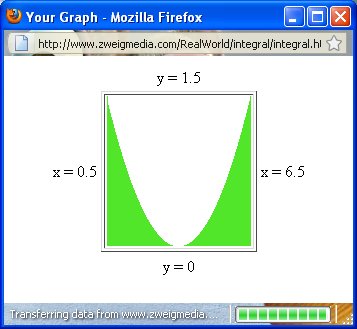
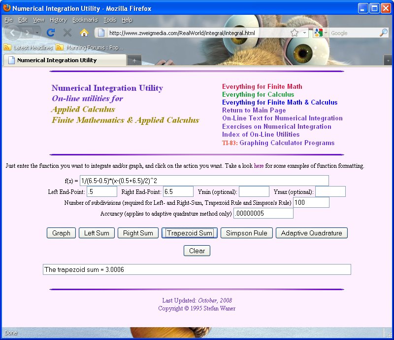
If you want to learn how the above standard deviation formulas are derived go to http://primepuzzle.com/tunxis/statistics/discrete-uniform-distribution.html. Note: the proof for the *continuous* case requires a knowledge of calculus. If you don't know calculus, don't worry about it. Calculus involves computing the area under a curve y=f(x) between two values of x. This is called "integration." (It also involves something called "differentiation" but we won't get into that here.) In our case, the "standard deviation function" is y=f(x)=1/(6.5-0.5)*(x-(0.5+6.5)/2)^2 where ^ means "raise to the power of." This can be seen to = 1/6*(x-3.5)^2. There is an online integration program at http://www.zweigmedia.com/RealWorld/integral/integral.html. I used it for this particular problem and captured both the graph of this function and the screen that shows the area under the curve. This area came out to be *very* close to 3. We need to take the square root of this to get the standard deviation (since 3 is the variance). The square root of 3 is about 1.73205.

- Lee